Introduction
Each year, the Cruising Club of America holds a weather seminar where they invite many experts to discuss a wide range of weather topics of interest to sailors. The videos from the 2020 weather seminar, which was held on February 29, have been made available here.
After watching a couple of the videos, I thought it would be worthwhile posting some of the discussion, as it may be of interest to sailors using LuckGrib.
I’ve selected a couple of the videos to focus on and have transcribed the portions that I was most interested in. As the videos are posted on YouTube, I believe they are in the public domain and that my transcribing this content will not violate any copyright laws. I also believe the portions I have transcribed are accurate.
Stan Honey, on GFS and ECMWF
Stan Honey was one of the invited speakers at the 2020 seminar. Stan Honey is a successful, professional offshore navigator. As noted on his Wikipedia page:
Honey’s track record as a navigator includes a victory in the 2005-06 Volvo Ocean Race onboard ABN Amro I and eleven wins in Transpac races across the Pacific Ocean. He has held the speed record for sailing around the World, and across the Atlantic and Pacific Oceans. He was named U.S. Sailing’s 2010 Rolex Yachtsman of the Year for his critical role in cutting the nonstop circumnavigation record to 48 days aboard the 103-foot French trimaran Groupama 3.
Stan’s opinion on topics related to ocean navigation carries some weight.
The video is interesting from start to finish. I encourage sailors to watch it all. He goes on to discuss weather routing later in the video, which is also very interesting.
| … my impressions now, and I think most navigators impressions now, of the GFS, is that its just as good. [as the ECMWF model] – Stan Honey. |
Stan Honey, discussing global weather models.
– Video time: 10m 11s. Global model discussion.
Global model examples. I won’t spend a lot of time on this because you’ve heard quite a bit earlier today. The GFS, in my experience, where people sail, meaning in areas of nice weather, the GFS has gotten extremely good. My recollection in the old days, was that the EC model and the GFS would kind of leap frog each other, one model would improve while the other model held still, and then vice-versa. The last time the GFS was by far the best was about 2010 - 2011. Then the ECM model got better, and has stayed better from 2012 until now, and my impressions now, and I think most navigators impressions now, of the GFS, is that its just as good. And I know that Joe [Sienkiewicz] doesn’t think that, and I know that some of the analysis that you see online indicates that that may not be the case, but for sailors, and we typically sail in areas of nice weather, and we typically only focus on the first three or four days of the forecast, I mean, that’s what really matters to us, the overall impression has been that the GFS, since the FV3 change, and other changes, has been kick-, you know, knocking it out of the box. That the GFS is doing a terrific job.
The GFS updates every 6 hours, you can get it in quarter degree, or .11 degree resolution. It runs for 15 days, its worth looking at for 8 days, its worth taking seriously for 6 days and you can take it to the bank for 3 days. [laughter.] And there’s another one in 6 hours.
The ECMWF is more complicated. Since 2012, I think from 2012 til 6 months ago, it was better. I think recently, in the last 6 months or so, the GFS has been extraordinary.
[continues with pricing and how that relates to racing rules.]
– Video time 14m 18s. More on ECMWF.
It [ECMWF] runs every 12 hours, it runs out for 10 days, and similarly, its worth looking at for 8 days, its worth taking seriously for 6 days and you can take it to the bank for 3.
Note above where Stan mentions the time frame:
I think recently, in the last 6 months or so, …
GFS was upgraded on June 12, 2019, to version 15.1, which is the version introducing the FV3 core and many other changes.
One minor correction: Stan mentions that GFS is available at 0.11 degree resolution. I don’t think this is true. It is calculated, internally at 1/8th degree resolution, but that data is not published.
Joe Sienkiewicz, on GFS, ECMWF
Joe Sienkiewicz is the Chief of the Ocean Applications Branch, part of NOAA’s Ocean Prediction Center. Joe has been with the National Weather Service for more than 30 years, and in that time he has become an expert in a variety of aspects of ocean weather. Joe’s opinion on weather models is worth listening to.
Joe goes through an interesting comparison of some of the current global weather models, starting at 38m 20s into the video. For this comparison, he is using a measure of forecast skill, called anomaly correlation, for the 500mb height (P500), over the northern hemisphere excluding the tropics (NHX), at 5 days into the forecast (fh120.)
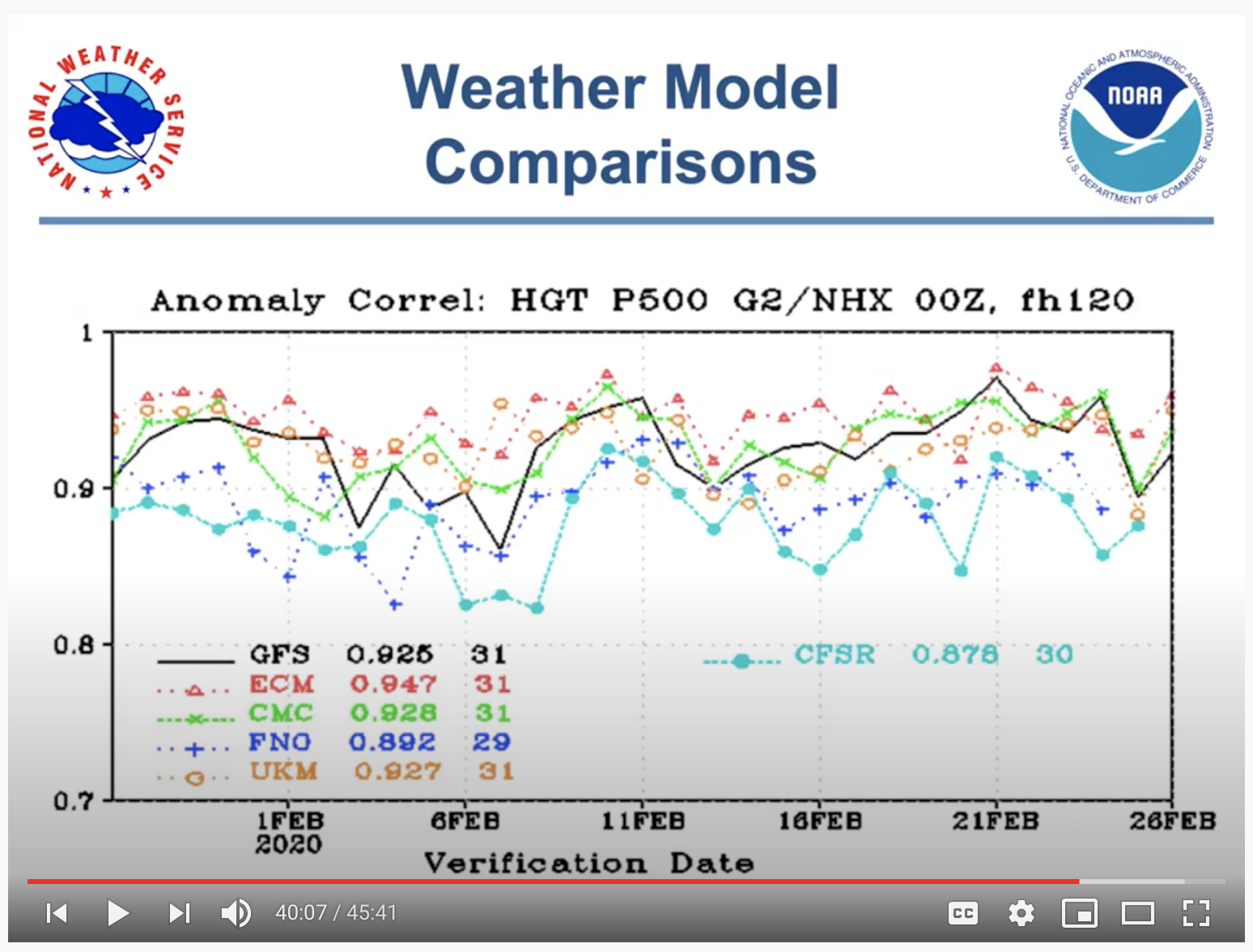 screen capture from 38m 20s of the video
Joe correctly notes that the ECMWF skill score, on this metric, is higher than GFS. Clearly, higher numbers are better, and the ECMWF values are higher than the GFS values, on average, on this image.
There is also something called a die-off curve:
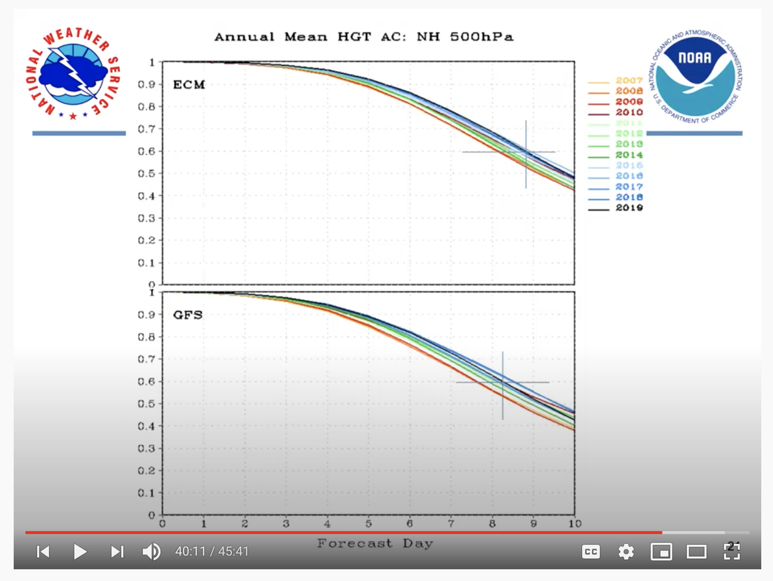 screen capture from 40m 17s of the video
Joe discusses die off curves and explains what the image is showing. To paraphrase, the image is showing the anomaly correlation (skill), over a forecast, averaged for a year, with each year displayed as a curve. The multiple curves are showing the evolution of the skill values in the weather models.
Joe mentiones that a skill value of around 0.6 is thought of as an accepted critical skill value. The point where ECMWF falls to the 0.6 skill value is at around 8.8 to 8.9 days. GFS is at around 8.2 days. Joe also mentions that the GFS and ECMWF are really similar to about day 5 and day 6 [41m 30s.]
I find this very interesting. Recall from Stan’s video where he said:
[GFS is] worth looking at for 8 days, its worth taking seriously for 6 days and you can take it to the bank for 3 days.
That statement is backed up from the graph shown above.
I have tried to find a way of putting this into context. I found a paper called Review of GFS Forecast Skills in 2012 which contains a review of this same skill score, over the period 1984 to 2012. (If anybody finds a more recent paper doing this comparison, please let me know.)
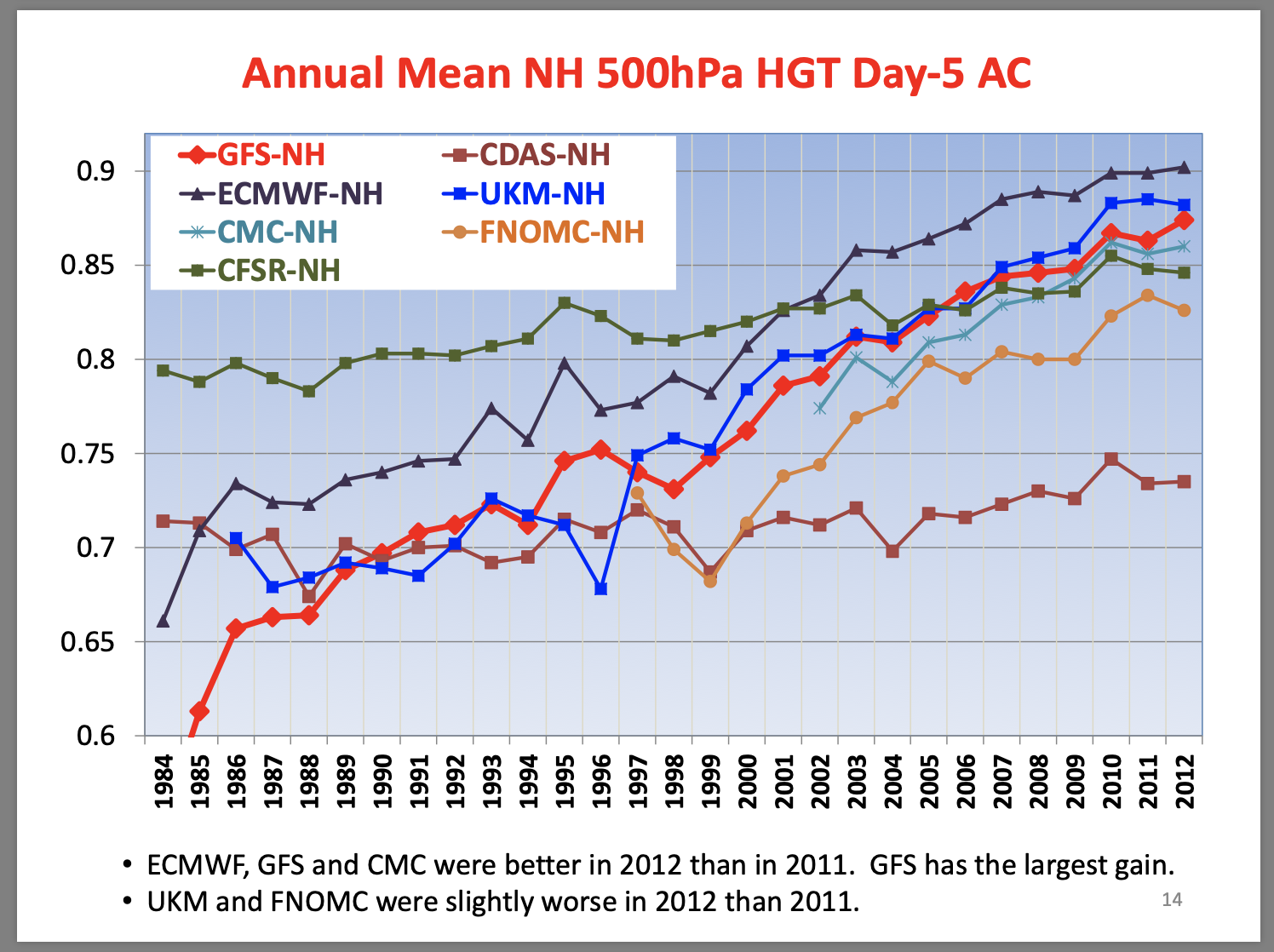 screen capture from page 14 of above PDF
Note how the weather models are all improving over time. Note that the current GFS skill score, from Joe’s first slide shown above, is 0.925, above all of the models in the image above.
Clearly higher skill values are better. The weather models are better now than they have ever been. Neither GFS or ECMWF offer a lot of forecast skill for the later forecast hours. ECMWF is slightly better than GFS, but the difference can be subtle. I would bet, although I have not seen data supporting it, that todays GFS is better than ECMWF from a few years ago.
From Joe’s first slide, for the day 5 forecast, most often the ECMWF forecast is showing higher skill, but there are some forecasts where GFS is better. When you are on the water, how do you know which forecast is going to be better? As neither weather model is perfect, does it really matter? We need to accept that for longer forecast hours, there is uncertainty in the models, and plan accordingly. The first few days, for both GFS and ECMWF are very good.
LuckGrib allows you to study weather model uncertainty. (Continue reading, as David Burch discusses model uncertainty below.)
One more data point that readers may be interested in: the ECMWF charges around €140,000 per year for access to their global model. GFS is freely available. (Do you want to create your own weather service? You can start by looking through NOMADS.)
Stan Honey on HRRR
Returning now to the first video, where Stan Honey discusses weather related topics. Stan spent a little time discussing mesoscale models.
| Definition of ‘mesoscale’: an intermediate scale, especially that between the scales of weather systems and of microclimates, on which storms and other phenomena occur. |
LuckGrib has been offering the HRRR model since early 2017. Its updated hourly, has forecasts out to 18 hours, and has a 3km resolution.
– Video time: 15m 15s. Mesoscale models.
Joe mentioned it, but I would like to underline it, the HRRR, I guess affectionatly known as the “hurr”, is extraordinary. Its absolutely unique in the world, and its in the process of changing our sport, not necessarily for the better, but the HRRR is amazing. It updates every hour, it runs for the continental US and its stunning.
[Some racing related discussion omitted.]
And just as a couple of examples, the HRRR will absolutely perfectly predict every single day whether the westerly in San Francisco bay is going to fill from the gate or from the Berkeley shore. It nails it. In Newport Rhode Island, which is one of the toughest areas to navigate, it will predict within 10 minutes, when the morning drainage breeze is going to glass off and when the sea breeze is going to fill in. And then in Newport Rhode Island, as you all know, once the westerly, the sea breeze, has filled in, as long as the wind is twisted vertically you want to go left, but as soon as the twist is out of the wind you want to go right. Well the HRRR will predict that transition within about 10 minutes. So the HRRR is just an extraordinary model, and I think it really will change the sport of sailing. And I think it has already in the US, and I think people are crazy if they don’t find a routine way to download that every hour, because its really an astonishingly effective tool.
and then again, a bit later:
Video time: 17m 15s. Predict Wind PWG and PWE
[early discussion omitted. Mainly update frequency]
Those models are pretty good, but the fact that they only update every 12 hours make them much, much less useful than the models that update more frequently.
David Burch on model uncertainty
David Burch is an author, navigator, sailor and has been active in the marine community for decades. Among many other books, David is the author of Modern Marine Weather, which is highly recommended. Many of you should know of David, as he has been active in this community for decades.
Rather than transcribe his talk, I would like to highlight several portions of it. You are, of course, encouraged to watch the talk in its entirety.
At 3m 20s into the video, David talks briefly of statistical models, the National Blend of Models and Standard deviation.
At 9m 30s into the video, David talks on the comparison of PRMSL and MSLET.
If you have been following LuckGrib closely, you will have noticed that I switched the sea level pressure field in GFS from PRMSL to MSLET in August, 2018. I believe that LuckGrib was one of the first weather providers to do this. I spent a considerable amount of time doing the research into the switch, and then publishing it. Since posting that article, MailASail has made the same switch, as has SailDocs. MailASail made the switch after reading my article. I don’t know why SailDocs switched from PRMSL to MSLET, although I would be interested in knowing.
At 35m 15s David starts to discuss ways to study model uncertainty. GEFS and the National Blend of Models (NBM.)
The NBM Oceanic model provides probabilty wind values, which is a way to see the spread of values among many of the available forecasts (the blend takes as input the GFS, ECMWF and many other models.) There are also several models which provide statistics on certainty, through the standard deviation. Standard deviation is available in GEFS, CMC ensemble and NBM Conus.
As far as I know, LuckGrib is the only app and service which support, and provide the standard deviation values. Additionally, I also believe that LuckGrib is the only weather provider, serving the marine community, providing access to any of the excellent NBM models.
– Video time: 37m 50s. Discussing NBM Oceanic
…in one sense, I think one could argue, that this might be the best long term ocean data available, period, in the world, any country.
At 38m 25s David compares a deterministic model, the GFS, to NBM Oceanic.
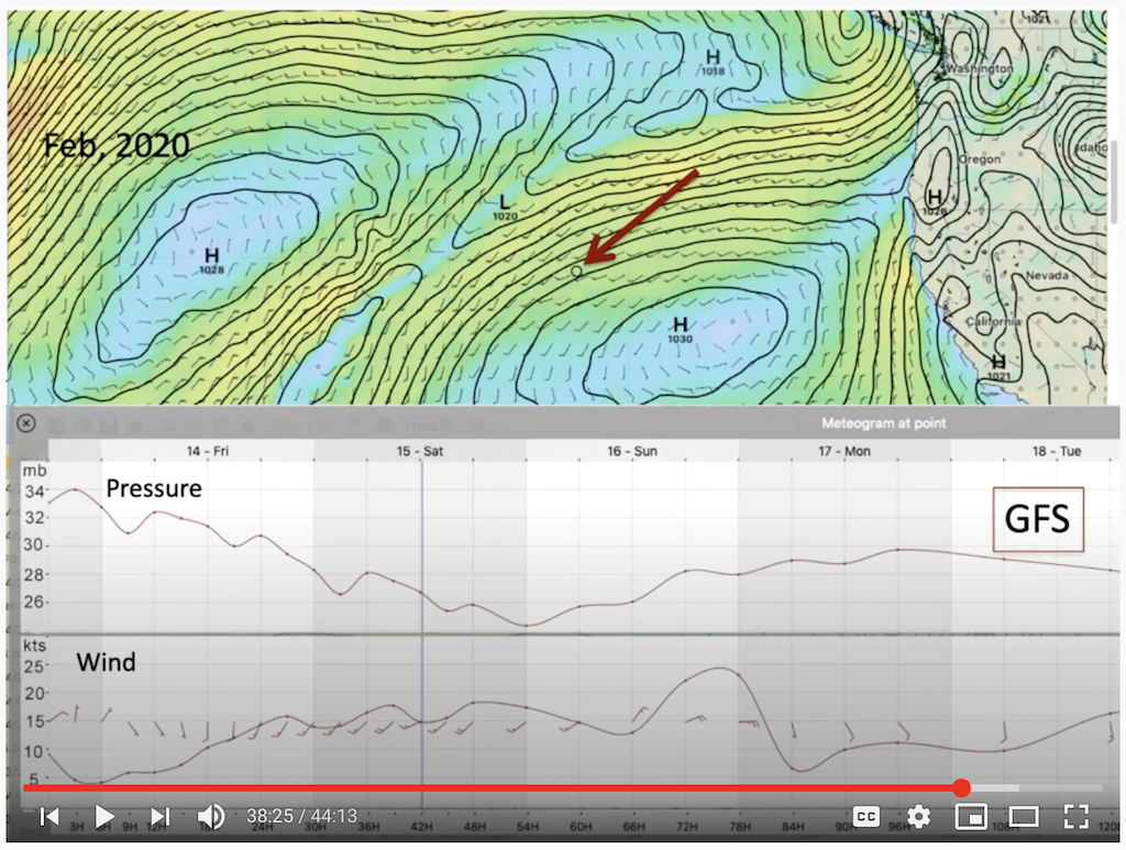
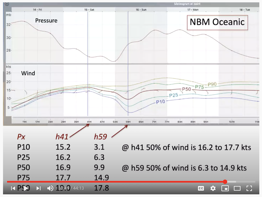
David’s discussion of this comparison is interesting.
A bit later, at 40m 19s, David discusses the NBM Conus model, and its recently introduced parameter for the standard deviation of wind.
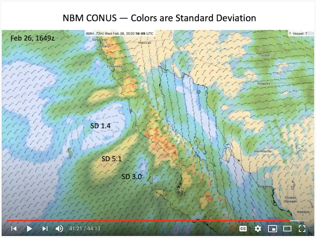 screen capture from 40m 19s of the video
Thanks to the Cruising Club of America
Thank you to the CCA for making these videos available!