General introduction
The support for ensemble models in both the LuckGrib application and in the LuckGrib server cluster has been greatly improved.
Before proceeding much further, lets see a few images.
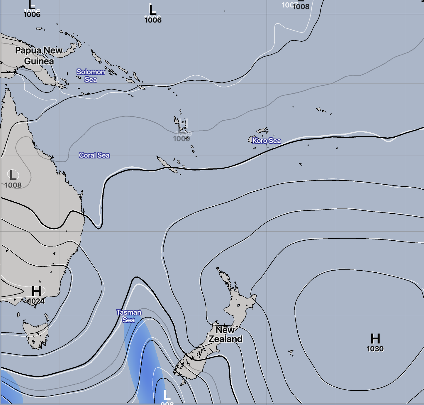
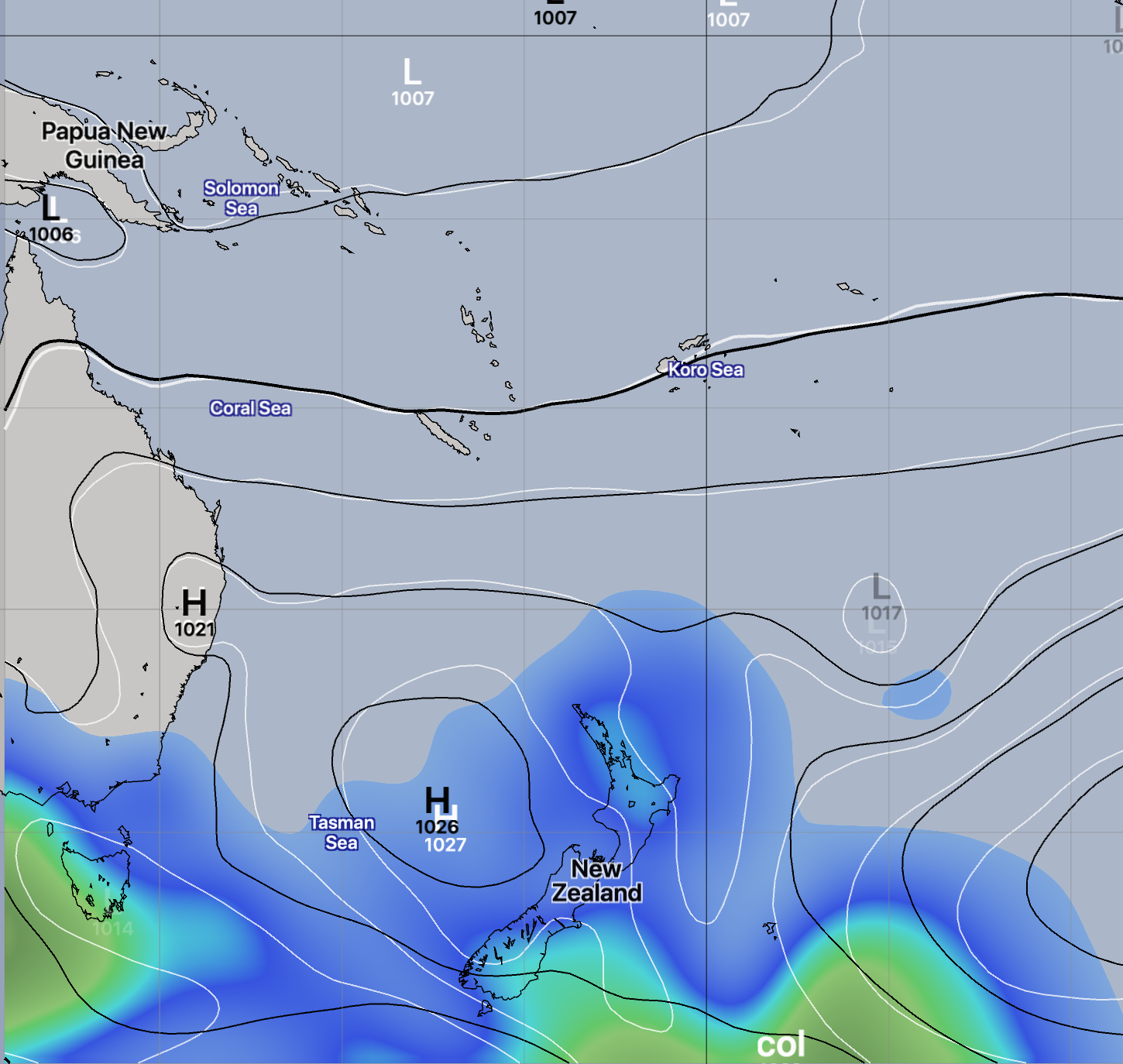
These two images are from the GEFS model, the GFS Ensemble. The images are showing the ensemble average sea level pressure as black contours, the original GFS control sea level pressure as white contours and the shading is showing the standard deviation present in the ensemble at the forecast hour.
The image on the left is showing, as you would expect, that the ensemble forecasts all have close agreement (small standard deviation) and that the ensemble average agrees closely with the GFS input.
On the right, 4 days into the forecast, the GFS and ensemble average are starting to diverge, and the standard deviation among the ensemble is growing. Note that the agreement among the ensemble and the original GFS input is very close in some areas and growing more divergent in others.
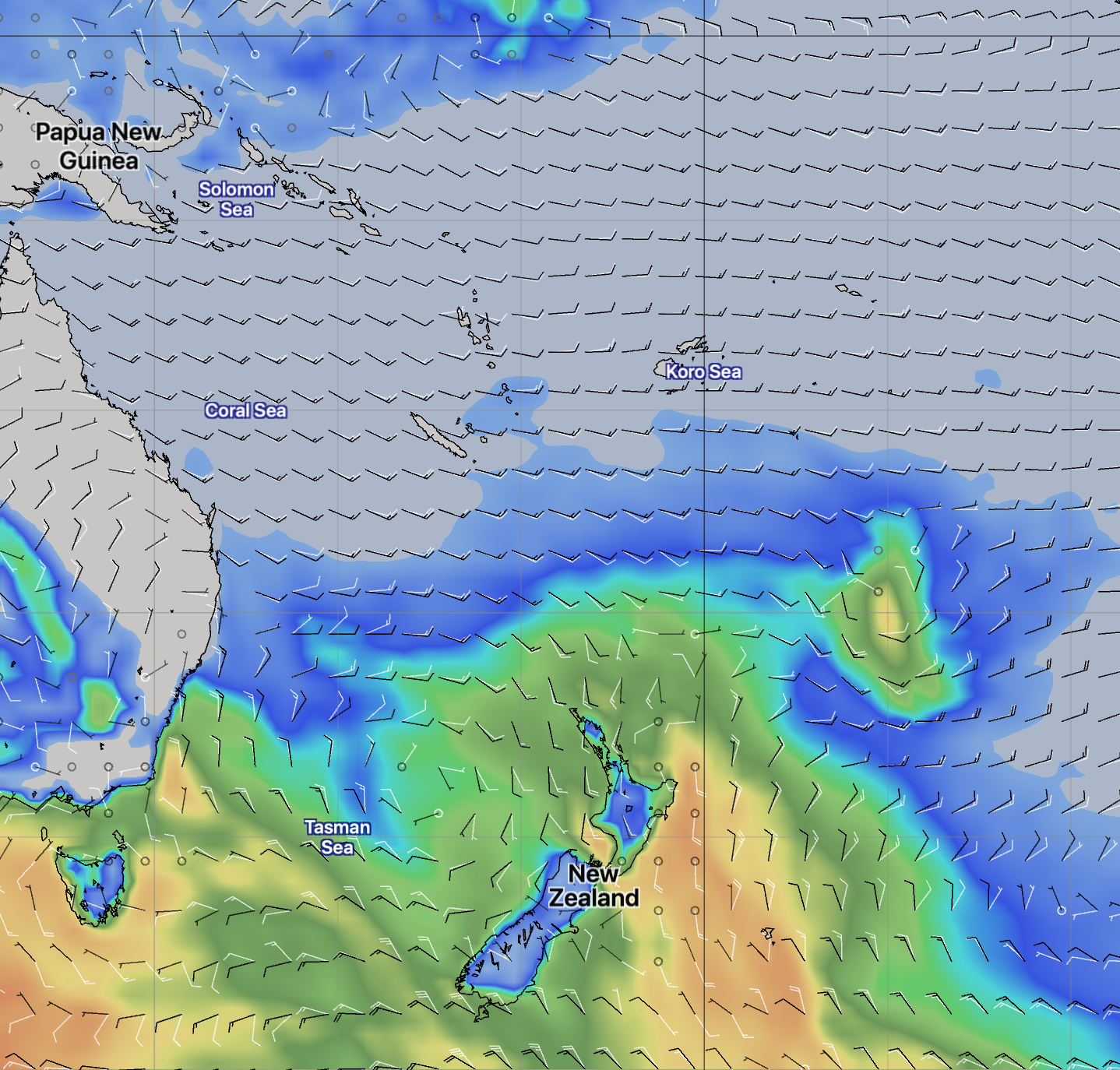
This image above is showing the GEFS ensemble average wind speed and direction as black wind barbs, the GFS control member wind in white and the standard deviation for wind as the color image. Note that this image gives you much more information about areas where you may trust the forecast information than is present in a deterministic model run, such as pure GFS.
The area east of the NE coast of Australia looks very stable, and I would have pretty high trust for those wind forecasts. The area east of New Zealand, even four days into the forecast, looks very difficult to predict. The winds are ranging from 0 to 20 knots in some area, with the wind direction entirely unpredictable.
If you were looking at a pure GFS forecast for this forecast time, you would not know that this level of uncertainty existed, in some areas, for these weather systems.
Ensemble standard deviation images are able to show you the uncertainty present in the ensemble forecast. This is an important point! When you are looking at a 4 day forecast from most weather models what you are seeing is one of the possible solutions, without any knowledge of how certain the forecast is of its solution.
Viewing ensemble standard deviation information shows you the agreement among the ensemble, and it appears that this can be extremely valuable to know.
Introduction to ensemble models
Briefly, and somewhat simplistically, there are two main types of GRIB models available: deterministic and ensemble.
In a deterministic model, the computer weather model is run and its best effort is made to produce an accurate forecast. The result of a deterministic model is its best guess at an answer for each point and forecast time.
In an ensemble model, the computer weather model is run multiple times, each with slightly different input or slightly tweaked model physics. The result of an ensemble run is a series of different possible forecasts. With GEFS and CMC, two of the ensemble models supported by LuckGrib, there are 21 possible answers provided: the original control member (GFS or GDPS) as well as the 20 perturbed forecasts. The ECMWF public domain ensemble uses 52 members in its ensemble.
The general idea behind an ensemble forecast is that all of the processes involved in generating a numerical weather prediction are imprecise. The process of capturing the initial atmospheric and ocean conditions, which is used to initialize the weather model, is imprecise. The simulation of the physics involved in how the atmosphere evolves over time, given some set of conditions, is imprecise.
When a series of imprecise operations are performed on a dynamic model such as a computer generated weather forecast, the results can end up being wildly wrong - the errors tend to increase over time.
Every attempt should be made, and is being made, to generate more accurate deterministic models. The various agencies are constantly striving to improve all areas of their weather forecasts.
However, an ensemble model embraces the idea that we will never be able to perfectly accurately capture the initial conditions or simulate the weather and that producing a range of possible outcomes and analyzing that suite of solutions can lead to greater insight into weather systems.
An ensemble model may generate 20 different forecasts, any of which could be the best fit to the actual conditions. After all of these potential solutions are generated, the model will perform some statistical analysis and create the average and standard deviation among the results.
One study I read mentioned:
… In addition, the high resolution control member is the best member of the ensemble ONLY ~ 5 to 7% of the time for all lead times (forecast hours).
Until doing this work on ensembles, I had assumed that the original GFS input to GEFS was somehow much better than the 20 generated ensemble members. This appears to have been a false assumption on my part.
There are studies which show that ensemble models are more skillful (more accurate) than deterministic models once you advance in the forecast beyond somewhere around 4 days. Forecasts shorter than 3 to 4 days may benefit from using the deterministic solution, but beyond that, the ensemble mean may be the more accurate solution. This is very interesting, and applies to all deterministic models.
We each probably have some rule of thumb we use, such as:
“GRIB weather forecasts are generally accurate for the first three or four days and then they all fall apart…”
– some random rule of thumb, by someone
In the above rule, the threshold for how far you can trust a forecast may vary depending on the model; the weather being forecast; the region of the world and other factors.
By viewing the additional information present in an ensemble model, we do not need to use such a crude rule of thumb. We can start analyzing the information provided by the ensemble model to know where to place more or less trust in a forecast
What’s new?
Until this version of LuckGrib only the ensemble mean (average) has been supported. Now, the ensemble mean, standard deviation and the control member information is available and supported in the app.
This information is present for all of the GRIB parameters in the model: sea level pressure, wind, rain, temperature, relative humidity, as well as the various levels: 850mb, 500mb, 250mb.
Here are a few more images:
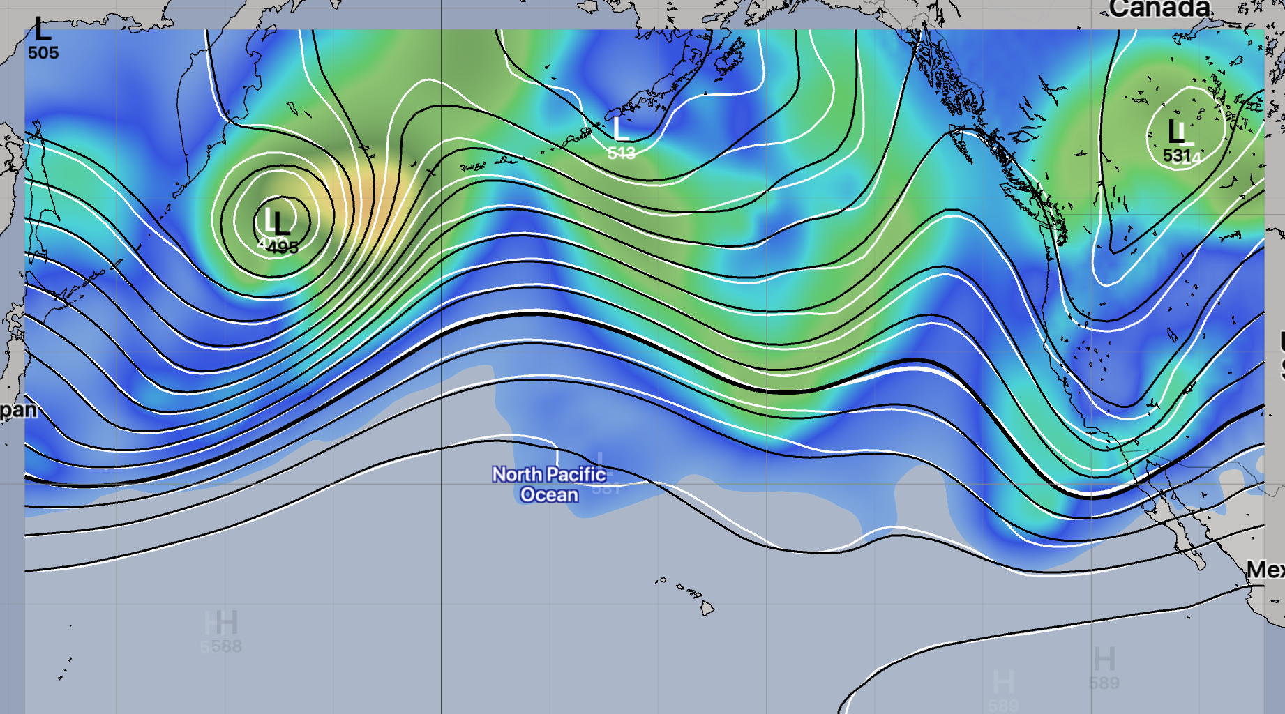
The image above is showing the 96H forecast, showing 500mb ensemble mean in black, 500mb control member in white and standard deviation as a color image. There is pretty close agreement among the ensemble for this forecast.
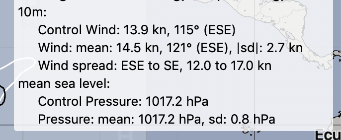
The information window now includes the ensemble mean, control and standard deviation information. For GEFS and CMC, wind standard deviation is provided as a vector, the magnitude of that vector is shown above. Also shown is the one standard deviation spread of the wind direction and magnitude.
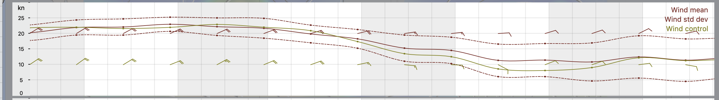
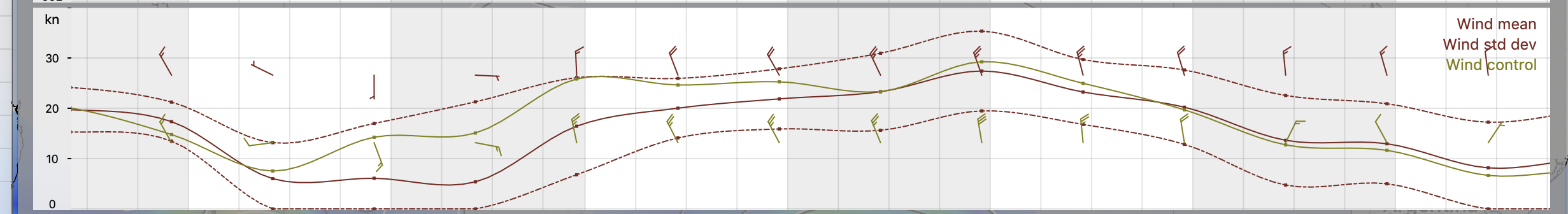
Two meteogram images are shown, the first east of Hawaii, in trade wind conditions. The second is off the coast of California, in an area of greater uncertainty. The meteogram is showing, as dotted lines, the one-deviation bands which surround the ensemble mean.
Conclusion
This new ensemble statistical information is potentially very valuable to people interested in analyzing longer range weather forecasts. It may also have great value in evaluating forecasts in the earlier forecast hours, as shown, even at 96H (or earlier.)
I believe LuckGrib may be unique in offering this data to weather forecasters in an easily available application.
I look forward to hearing from others on what they think of this new data. Please forward any comments or suggestions you may have.