Introduction:

As mentioned on the home page of this site:

LuckGrib takes its cues for the presentation of weather graphics from professional weather forecasting organizations, such as NCEP. Smooth contours. Highs and lows positioned accurately. Streamlines available to show winds in the tropics.

One of the technologies that is instrumental in achieving those goals is the technique LuckGrib uses to interpolate the data it finds in GRIB files.

Background:

Recall that a GRIB file is a file composed of various records, each of which describes a single parameter at a particular point in time. Each record describes a reference time, which is the time the forecast was created, as well as a valid time, which is the time this particular record is valid for. Along with the time information, each record contains data describing the grid for the data (the latitude and longitude for each data point) as well as the actual data itself.

The data for a GRIB record is simply a series of values, arranged in a grid. Each data point is a value - for example, if the record is recording the mean sea level pressure then one of the values may be 1020.1. Each of the values is independent and describes the value for the record at that particular point.

Its very simple. GRIB delivers a grid of values. Its up to the GRIB viewing software to read, interpret and generate graphics to represent the data. This is where the different GRIB viewers start to show their differences - and where LuckGrib starts to shine.

The essential point, for purposes of this discussion, is that the GRIB file defines grid point values - what happens in-between these points is not defined by the standard, and each GRIB viewer is left to implement its own technique for what to do if it needs to display a value for a record at a point that is not on the grid.

The process where you have a grid of data and you create intermediate points is called interpolation. The application interpolates the surrounding data in order to generate these intermediate values. The various GRIB viewers use different interpolation techniques, and the quality of these techniques is apparent in the graphics that they display.

LuckGrib uses a very robust and high quality interpolation technique.

The grid used in the example:

For purposes of this example, I have chosen a somewhat random GRIB file, which contains mean sea level pressure and wind data. If you would like to follow along, you can download the example GRIB file.

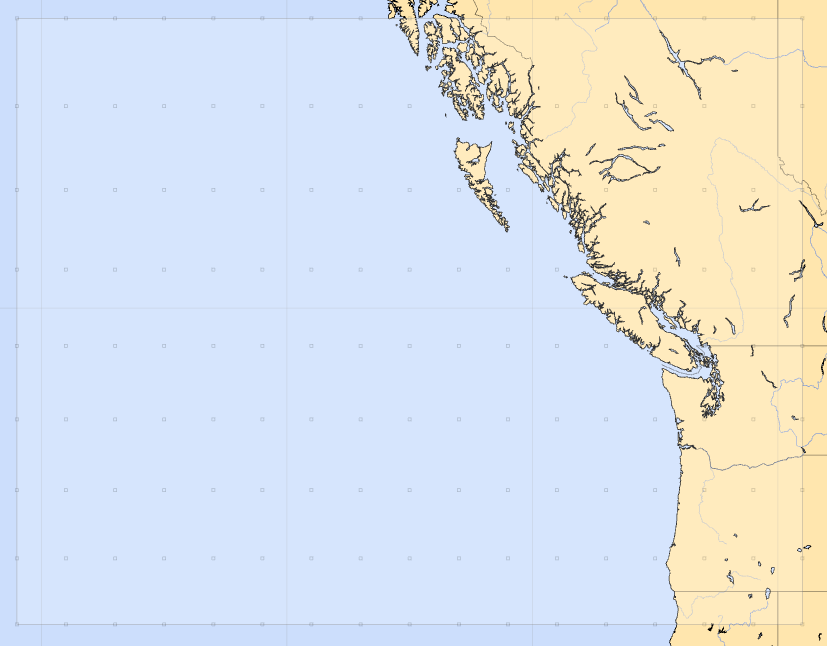
This first image is created in LuckGrib, and shows the grid that data in the file is created on. Each of the little squares in the image above represents a point where an actual GRIB data point is defined. Any value you see displayed in-between these grid points is an interpolation point. (Notice that in this example, the grid is fairly widely spaced - this would be typical of a file you download while on a sailboat on a passage.)

Example contours:

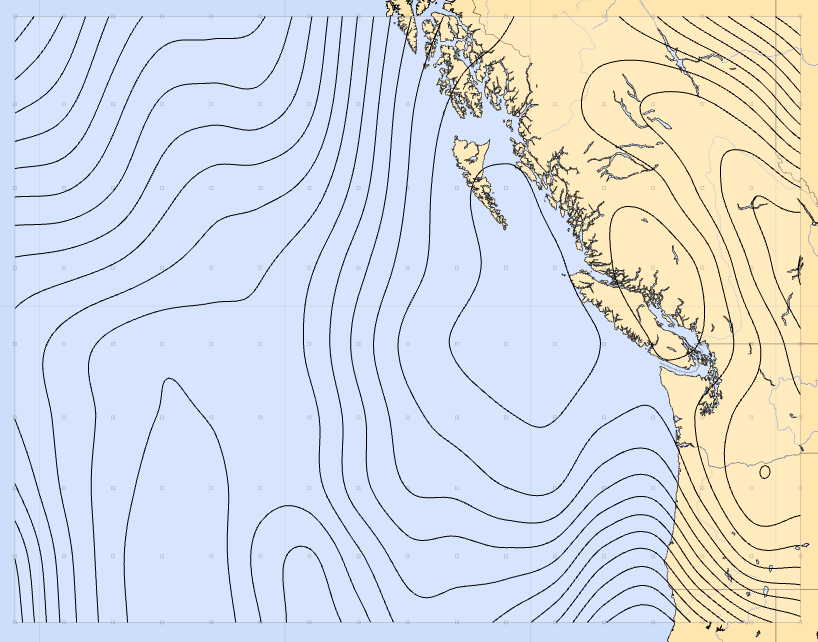
LuckGrib generated image. (The Default contour interval has been changed to 1mb from its normal 4mb.)

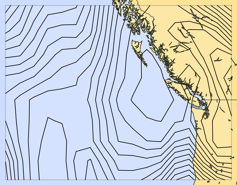
zyGrib generated image. (The default zyGrib colors for land and sea were modified to more closely match LuckGrib, in order that the images would be more similar. The contour interval has been set to 1mb, just as in the LuckGrib image.)

While this example presents an image created by zyGrib, it is not meant to pick on zyGrib. I believe the contours zyGrib generates are typical of most of the GRIB viewers available. If you have access to a different GRIB viewer and can compare its contours to those of LuckGrib, please do so. Download the file above and try to replicate the positioning of the view. If you could send the results to me, I would appreciate it.

Results:

It should be clear that the contours generated by LuckGrib are much better. They are more accurate and follow the principal outlined at the start of this article. You don’t see professional weather forecasters publishing contours composed of straight line segments, why should you put up with these types of contours in your GRIB viewers?

One response to the higher quality of LuckGrib’s contours may be: so what? While LuckGrib generates higher quality, smooth contours, and other applications commonly generate contours composed of rough line segments - the poorer quality image still conveys approximately the same information.

The author of LuckGrib believes that having LuckGrib create pleasing and natural images is important. High quality images are easier to work with, and that is what LuckGrib strives to achieve.

The pressure contours in the real world will not exactly correspond to either image - but there should be no question that the smooth contours will be a much closer match to what is happening in the real world than the contours composed of crude line segments.

Back to the topic - interpolation:

There are two separate processes related to the high quality of LuckGrib’s contour generation:

• the high quality of the interpolation used
• the high quality of the contour generation algorithm

This article focuses on the interpolation portion of this process.

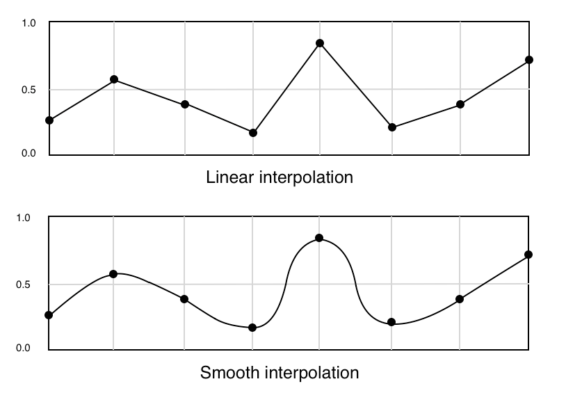
So, what exactly is interpolation? Consider eight values along a line. These may be eight values along a line of latitude, for example. The values at the grid points is defined by the GRIB file - however, the values in-between these given points is the result of the type of interpolation used.

I will simplify this discussion, by considering two main families of interpolation:

• linear
• smooth

(There is a wide variety of ways to implement smooth interpolation, that discussion will be avoided, as it is quite deep and technical.)

Many GRIB viewers appear to implement some sort of linear interpolation. Given two adjacent values, to calculate a value in-between them, there is an assumption that the values vary in a linear manner - i.e. each data point is connected by a line to its neighbors. If you do a linear interpolation, a graph of the values looks something like the example above.

Smooth interpolations are more difficult, complex and costly - however they are a closer match to the way things work in the actual world. A smooth interpolation creates smoothly varying values.

In order to create smooth contours, the application must perform some sort of smooth interpolation. I believe most GRIB viewers do not do this, and that is likely a large part of the reason many other GRIB viewers produce such poor quality contours.

Note that an application could implement a smooth interpolation process and use a simple contour generation algorithm to end up with simplistic, angular contours. In order to achieve smooth contours, the application must implement both smooth interpolation and a high quality contour algorithm.

The important point is: the weather that GRIB files are modeling, the weather that we sail around in and experience everyday, is not modeled well by linear interpolation. In general, changes in the weather happen smoothly. GRIB viewers which use linear interpolation are introducing artificial artifacts into their graphics. The author of LuckGrib has gone to a great deal of trouble to create a high quality, fast, interpolation scheme, and the results of this work are easily visible to anybody who uses the application.

Interpolation field:

The image above shows eight values along a line, and how how those values could be interpolated across that line. However, GRIB files are composed of a two dimensional grids of values. LuckGrib takes these two dimensional grids and creates an interpolator which operates in two dimensions, calculating a smooth interpolation across this grid. The result is a two dimensional field, which is defined at every point.

LuckGrib takes a very flexible approach to creating its field interpolators. You are able to create a field interpolator for all GRIB parameters, and indeed, this is done for you automatically.

All records in LuckGrib have one of these high quality, smooth, two dimensional field interpolators attached to it, and this field is used in the calculation and presentation of all of the data in the application. If you move your cursor to one of the grid points, then the value for the field at that point is guaranteed to be the value from the GRIB file. As you move away from the grid points, the interpolation is performed in a smooth manner.

Smooth interpolation, everywhere:

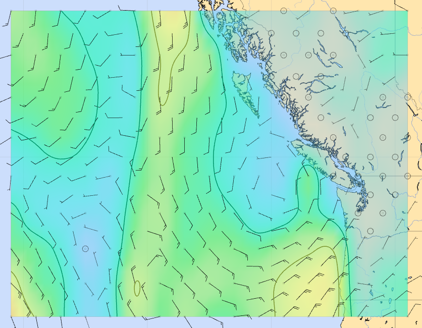
This image is one last example of smooth contours. In this case, the contours shown are contours of wind speed. There are two contours shown, one for 10 knots and one for 20 knots. These contours separate areas where the wind speed is less than 10 knots from areas where the wind speed is above 10, and again for where the wind speed is above 20 knots.

The techniques used in the interpolation process are completely general in the application, as are the techniques used to generate contours. All GRIB records are smoothly interpolated and you can generate a contour image for any of the GRIB parameters.

Wind speed interpolation will be discussed in more detail in a subsequent tutorial.

The bottom line…

LuckGrib creates high quality, accurate images, in real time. While the processes and algorithms used to achieve these high quality images are complex and computationally demanding, LuckGrib is a very high performance application.

LuckGrib uses a powerful interpolation technique which tries to create the highest quality two dimensional fields possible. These high quality fields more closely represent what we experience in the real world than poorer (and faster) approximations.

The technology behind the scenes to make all of this work is complex - but using the application isn’t.